In this blog post, we will explore the concept of Gaussian Mixture Models (GMMs). These models are intuitive and widely applicable in various domains such as image segmentation, clustering, and generative modeling.

Introduction to GMMs

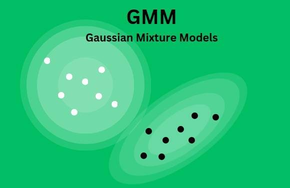
Gaussian Mixture Models are used to model an overall distribution through multiple Gaussian distributions. They are a powerful tool for capturing, estimating, and clustering parts of an overall distribution as locally Gaussian-distributed. GMMs are unsupervised models, meaning they do not need to know the specific Gaussian distribution a data point belongs to in advance.

Example of GMM

Here’s a simple example to illustrate GMMs:

1
2
3
4
5
6
7
8
9
10
11
12
13
14
15
16
17
18
19
20
21
22
23
24
25
26
import matplotlib.pyplot as plt
import numpy as np
from scipy import stats

# first gaussian
mean1 = 0
standard_deviation = 1
x = np.arange(-10,10,0.1)
y1 = stats.norm(mean1, standard_deviation)

# second gaussian
mean2 = -2.5
y2 = stats.norm(mean2, standard_deviation)

# third gaussian
mean3 = 2.5
y3 = stats.norm(mean3, standard_deviation)

# overall plotting
plt.plot(x, y1.pdf(x), '--', c='gray')
plt.plot(x, y2.pdf(x), '--', c='gray')
plt.plot(x, y3.pdf(x), '--', c='gray')
plt.plot(x, y1.pdf(x)+y2.pdf(x)+y3.pdf(x), c='black')
plt.xlabel('Coordinates')
plt.ylabel('Density')
plt.show()

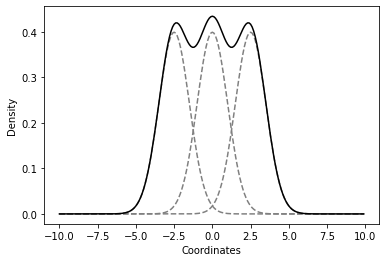
This example shows three Gaussian distributions fitting an overall distribution, with the black line representing the combined distribution.

Application of GMMs

GMMs have numerous applications, including:

• Image segmentation
• Multi-object tracking in videos
• Audio feature extraction

They are particularly useful for multimodal distributions, where multiple peaks are present. These peaks can be modeled using multiple Gaussian distributions.

Mathematical Formulation of GMMs

To represent GMMs mathematically, we need to understand three types of parameters:

1. Mixture Weights (\(\phi\)): indicate the probability that a point belongs to a specific Gaussian component \(K\).
2. Means (\(\mu\)): the centers of each Gaussian component.
3. Covariances (\(\mathbf{\Sigma}_i\)): describe the spread and orientation of each Gaussian component.

The probability density function for a GMM is given by:

where \(\mathcal{N}(\mathbf{x}\vert\mathbf{\mu}_i, \mathbf{\Sigma}_i)\) is the multivariate Gaussian distribution.

Training the GMM: Expectation-Maximization algorithm

The EM algorithm is used to find the maximum likelihood parameters of a GMM, especially when there are latent variables influencing the data distribution.

Steps of the EM Algorithm

1. Expectation (E-step): Estimate the latent variables.
2. Maximization (M-step): Maximize the parameters based on the current estimates of the latent variables.

In the particular case of GMMs, if one considers the maximum likelihood, we should maximize:

with respect to \(\theta = (\phi_i, \mathbf{\mu}_i, \mathbf{\Sigma}_i)\). However, two problems arise by doing so: 1) we can have very high (arbitrarily large) likelihood when a single Gaussian explains a point; 2) an unlimited number of solutions is acceptable up to permutations. Instead, if we do introduce a latent variable \(z\), then one can consider that the mixture model generates the data by first sampling from \(z\), and only then we sample the observable data \(\mathbf{x}\) from a distribution that does depend on \(z\), meaning:

In mixture models, the latent variables are easily interpreted as being the different components of the data distribution, i.e. \(z=c\) .

Let us try to optimize \(\ln p(\mathbf{x})\) for the set of parameters \(\theta\) by integrating over the latent variable

This means that the derivative of the marginal log-probability \(p(\mathbf{x})\) is the expected value of the derivative of the joint log-probability, with the expectation on the posterior distribution. This formula is completely generic for any model with latent variables as we did not introduce any specificities related to GMMs. We have not given the full details of the derivation, but just keep in mind that we have used the known property:

It is rather tempting to equalize the derivative to zero for the particular case of the GMMs. Doing so, you end up with the optimum parameters that we are looking for. In particular, our two previous steps of the EM algorithm become:

E-Step:

M-Step:

These two steps define fully the EM algorithm for the GMMs with a random initialization of the parameters \(\theta = \left\{\phi_i, \mathbf{\mu}_i, \mathbf{\Sigma}_i\right\}\).

Clustering with GMMs

To use GMMs for clustering, follow these steps:

1. Train the model to obtain the parameters (means, covariances).
2. Assign each data point to a Gaussian component based on the probability \(r_{ni}\).

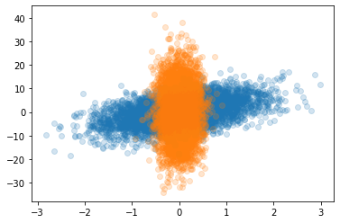
Let us first start by generating two non-trivial distributions:

1
2
3
4
5
6
7
8
9
10
11
12
13
import matplotlib.pyplot as plt
import numpy as np

mean = [0,0]
cov = [[0.05,0],[0,100]]
cov2 = [[0.5,0],[2,25]]

x,y = np.random.multivariate_normal(mean, cov, 5000).T
x2,y2 = np.random.multivariate_normal(mean, cov2, 5000).T

plt.scatter(x2,y2, alpha=0.2)
plt.scatter(x,y, alpha=0.2)
plt.show()

As you can see for the second example, we did not consider a diagonal covariance matrix. That’s also an interesting case, because there is some overlapping region that will definitely be challenging for the algorithm to understand.

The stopping criteria is related to the difference between the log-likelihood at a step \(𝑛-1\) and step \(𝑛\) being below a certain threshold. Meanwhile, until that threshold is not reached we continue updating the estimated parameters of the model. Let’s therefore built a class with a fit method.

1
2
3
4
5
6
7
8
9
10
11
12
13
14
15
16
17
18
19
20
21
22
23
24
25
26
27
28
29
30
31
32
33
34
35
36
37
38
39
40
41
42
43
44
45
46
47
48
49
50
51
52
53
54
55
56
57
58
59
60
61
62
63
64
65
66
67
68
69
70
71
72
73
74
75
76
77
78
79
80
81
82
83
84
85
86
87
88
89
90
91
92
93
94
95
96
97
98
99
100
101
102
class GMM():
    def __init__(self, n_components, n_iters, threshold = 1e-6, seed = 42):
        
        self.n_components = n_components
        self.threshold = threshold
        self.seed = seed
        self.n_iters = n_iters
        
    def fit(self, X): 
        """ Method that learns the parameters of the GMM
        """
        # initialization of the parameters
        old_log_likelihood = 0
        
        ## rni and weights, i.e. prior
        n_row, n_col = X.shape
        self.rni = np.zeros((n_row, self.n_components))
        self.weights = np.full(self.n_components, 1/self.n_components)
            
        # mean initialization
        np.random.seed(self.seed)
        choice = np.random.choice(n_row,self.n_components, replace=False)
        self.means = X[choice]

        # covariance matrix initialization
        shape_var = self.n_components, n_col, n_col
        self.covariances = np.full(shape_var, np.cov(X, rowvar=False))
        
        # start the main loop
        for i in range(self.n_iters):
            # compute first the log-likelihhod
            self.__log_likelihood(X)
            new_log_likelihood = np.sum(np.log(np.sum(self.rni, axis=1)))
        
            # run the E-M step
            self.__E_step(X)
            self.__M_step(X)
            
            # check convergence 
            if abs(new_log_likelihood - old_log_likelihood) <=self.threshold:
                break
                
            # if it did not converge, then update the log-likelihood
            old_log_likelihood = new_log_likelihood
                        
        
    
    def __E_step(self, X):
        """ Method that implements the E-step
        """
        #normalize over the different cluster probabilities
        self.rni = self.rni/self.rni.sum(axis=1, keepdims=1)
        
    
    def __M_step(self, X):
        """ Method that implements the M-step
        """
        phi_num = self.rni.sum(axis=0)
        phi_i = phi_num /X.shape[0]
        
        # means
        self.means = np.dot(self.rni.T, X)/ phi_num.reshape(-1,1)
        
        #covariances
        for k in range(self.n_components):
            diff = (X - self.means[k]).T
            cov_num = np.dot(self.rni[:,k]*diff, diff.T)
            self.covariances[k] = cov_num / phi_num[k]
        
    
    def __log_likelihood(self,X):
        """ Method to get the log-likelihood
        """
        for k in range(self.n_components):
            prior = self.weights[k]
            likelihood = multivariate_normal(self.means[k], self.covariances[k]).pdf(X)
            self.rni[:,k] = prior * likelihood
            
    
    def plot_component(self, X, title='Clusters'):
        """ Method that plots the different components assigned to the data points X
        """
        plt.figure()
        plt.plot(X[:,0], X[:,1], 'ko', alpha=0.01)
        
        delta = 0.25
        k = self.means.shape[0]
        x = np.arange(-4,4, delta)
        y = np.arange(-40,40,delta)
        x_grid, y_grid = np.meshgrid(x,y)
        coordinates = np.array([x_grid.ravel(), y_grid.ravel()]).T 
        
        col = ['green', 'red']
        for i in range(self.n_components):
            mean = self.means[i]
            cov = self.covariances[i]
            z_grid = multivariate_normal(mean, cov).pdf(coordinates).reshape(x_grid.shape)
            plt.contour(x_grid, y_grid, z_grid, colors = col[i])
            
        plt.title(title)
        plt.tight_layout()

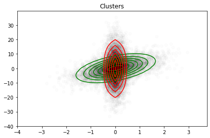
One can apply such class to our previous dataset and follows the figure below:

Challenges and Considerations

GMMs require specifying the number of components beforehand. Model selection criteria such as Akaike Information Criterion (AIC) or Bayesian Information Criterion (BIC) can help determine the optimal number of components. Additionally, the complexity of GMMs increases with the size of the dataset, particularly due to the covariance matrices. Simplifying assumptions, such as diagonal covariance matrices, can mitigate this issue.

In summary, Gaussian Mixture Models are a robust tool for modeling and clustering complex data distributions. Their ability to handle multimodal distributions makes them valuable in various practical applications.