Gradient descent is the workhorse of modern machine learning, but vanilla gradient descent often struggles with challenges like saddle points, ravines, and local minima. Momentum-based methods address these limitations through elegant mathematical principles that provide remarkable benefits. This post explores why momentum gradient descent works so effectively and has become fundamental to modern optimization algorithms.
The Physics of Momentum Optimization
Classical gradient descent performs a simple update: \(\theta_{t+1} = \theta_t - \alpha \nabla_\theta J(\theta_t)\), where \(\theta_t\) represents parameters, $\alpha$ is the learning rate, and $\nabla_\theta J(\theta_t)$ is the gradient. This approach navigates the loss landscape by always moving in the steepest downhill direction at each step.
Momentum gradient descent transforms this process by introducing a velocity term that accumulates previous gradients:
\[\begin{align} v_{t+1} &= \gamma v_t + \alpha \nabla_\theta J(\theta_t) \\ \theta_{t+1} &= \theta_t - v_{t+1} \end{align}\]Here, \(\gamma \in [0,1)\) is the momentum coefficient, typically around 0.9. This simple modification dramatically improves optimization.
The most intuitive way to understand momentum is through physics: imagine a ball rolling down a hill with friction. Standard gradient descent is like a ball in a thick fluid that can only move directly downhill at each point. Momentum is like giving this ball mass, allowing it to build up speed and continue moving even through small uphill sections.
This physical intuition can be formalized mathematically. Momentum optimization approximates a damped mechanical system governed by:
\[\begin{align} m\frac{d^2\theta}{dt^2} + c\frac{d\theta}{dt} &= -\nabla_\theta J(\theta) \end{align}\]Where the effective mass is related to the momentum coefficient by \(m \propto \frac{1}{1-\gamma}\). This means higher momentum values (closer to 1) give the system more inertia.
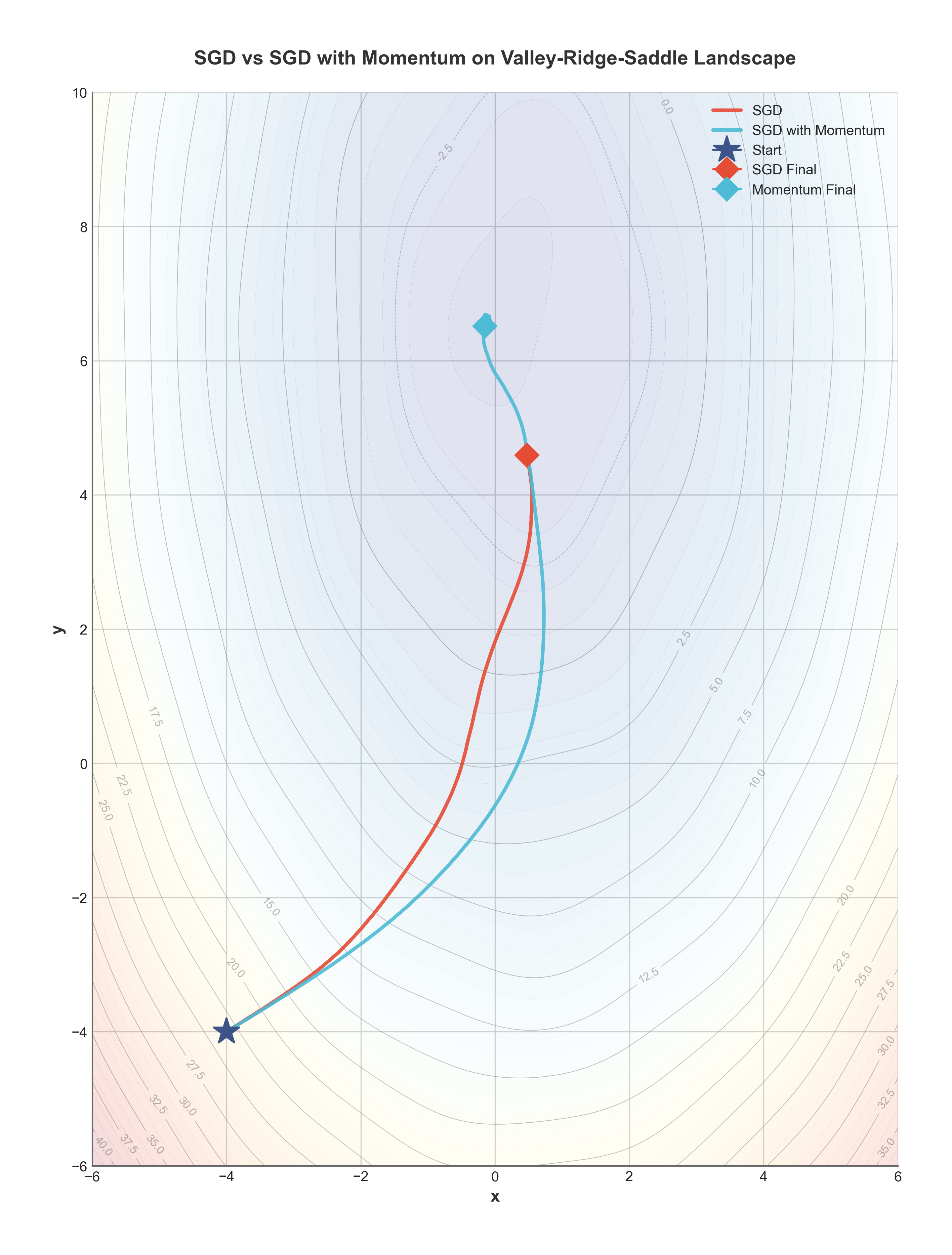
Phase space diagram showing trajectories of vanilla gradient descent vs. momentum in a 2D contour plot
Why Momentum Works So Well
Momentum acceleration provides three key benefits that dramatically improve optimization:
1. Smoothing Oscillations in Ravines
One of momentum’s greatest strengths is navigating ravines—regions where the loss surface is much steeper in some directions than others.
Consider optimizing a simple quadratic function \(J(\theta) = 100\theta_1^2 + \theta_2^2\). The surface is 100 times steeper in the \(\theta_1\) direction than in the \(\theta_2\) direction. Standard gradient descent zigzags inefficiently, oscillating wildly in the steep direction while making minimal progress in the flat direction.
Momentum naturally dampens these oscillations. The velocity accumulates in consistent directions while canceling out in oscillatory directions. This creates an effective “shortcut” through the zigzag path that vanilla gradient descent would take.
2. Escaping Saddle Points
Saddle points are locations where the gradient is zero, but the surface curves upward in some directions and downward in others. They’re extremely common in high-dimensional spaces like neural networks.
Standard gradient descent can get trapped at saddle points because the gradient vanishes. Momentum’s accumulated velocity allows it to cruise past these points, much like how a rolling ball doesn’t stop at the middle of a mountain pass.
This property is especially important in deep learning, where saddle points are far more common than local minima in high-dimensional parameter spaces.
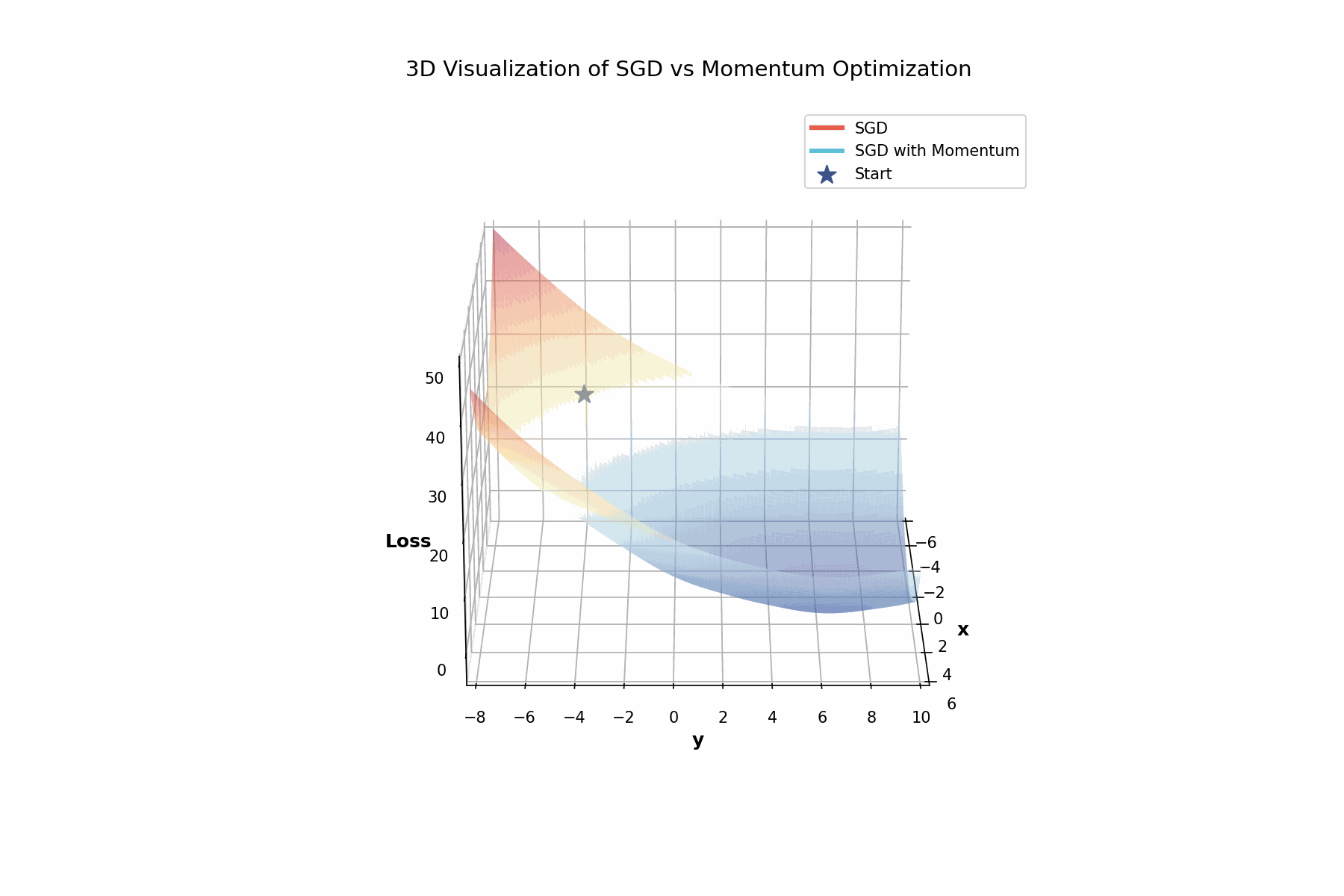
3D visualization showing how momentum helps navigate the complex loss landscape. The rotating view reveals the valleys and ridges that make optimization challenging.
3. Adaptive Effective Learning Rates
A less obvious benefit of momentum is how it creates dimension-specific effective learning rates. When we expand the momentum update recursively, we get:
\[\begin{align} v_t &= \alpha\sum_{i=0}^{t-1} \gamma^{t-1-i} \nabla_\theta J(\theta_i) \end{align}\]This shows that momentum computes an exponentially weighted moving average of past gradients. When gradients consistently point in the same direction, this sum grows, effectively increasing the step size. When gradients oscillate, they partially cancel out, effectively reducing the step size.
This natural adaptation happens automatically along different dimensions of the parameter space, creating a crude but effective form of preconditioning that adjusts to the local geometry.
Applications in Modern Deep Learning
The mathematical principles of momentum extend to more sophisticated algorithms used throughout deep learning. Nesterov’s accelerated gradient introduces a “look-ahead” evaluation:
\[\begin{align} v_{t+1} &= \gamma v_t + \alpha \nabla_\theta J(\theta_t + \gamma v_t) \\ \theta_{t+1} &= \theta_t - v_{t+1} \end{align}\]This subtle modification further improves momentum’s performance, especially for convex problems.
The widely-used Adam optimizer combines momentum with adaptive learning rates through a system of equations:
\[\begin{align} m_t &= \beta_1 m_{t-1} + (1-\beta_1)\nabla_\theta J(\theta_t) \\ v_t &= \beta_2 v_{t-1} + (1-\beta_2)(\nabla_\theta J(\theta_t))^2 \\ \theta_{t+1} &= \theta_t - \alpha \frac{\hat{m}_t}{\sqrt{\hat{v}_t} + \epsilon} \end{align}\]Here, the first equation is essentially momentum with $\beta_1$ as the momentum coefficient. Even the most advanced optimizers still incorporate momentum as a fundamental building block.
Practical Tips for Using Momentum
When implementing momentum in your own projects, keep these practical considerations in mind:
-
Default momentum value: 0.9 is a good starting point for most problems
-
Effective learning rate: With momentum, the effective step size is approximately \(\frac{\alpha}{1-\gamma}\) in the long run. For \(\gamma = 0.9\), this means the effective learning rate is 10× the nominal value! When switching from vanilla gradient descent to momentum, you may need to reduce your learning rate to maintain stability.
-
Improved generalization: Beyond faster training, momentum methods tend to find solutions that generalize better. The dynamics of momentum optimization naturally favor wider, flatter minima over sharp ones, which often translates to better test performance.
Momentum gradient descent represents one of the most profound advances in optimization for machine learning. Its elegant mathematical formulation combines insights from physics with optimization theory to create an algorithm that accelerates convergence, navigates challenging geometries, and improves generalization. Understanding these principles helps explain why momentum remains a core component of modern optimizers and continues to inspire new algorithmic developments in deep learning.
(Updated: )